AWS Quantum Technologies Blog
Demonstrating genuine multipartite non-locality on quantum processors using Amazon Braket
This post was contributed by Federico Hernán Holik, Andrés Camilo Granda Arango, Carlo Cuccu, Roberto Giuntini, Giuseppe Sergioli, Peter Komar, and Ishaan Pakrasi.
Quantum physics produces correlations that no classical theory can reproduce, and testing these differences on real hardware is now possible with cloud-based quantum computing through Amazon Braket. One of the most striking quantum features is non-locality: experiments violating Bell inequalities [1] show that no local hidden-variable model can account for quantum correlations.
In this post, we move beyond the standard two-qubit case and explore genuine multipartite non-locality (GMNL). We focus on inequalities designed to rule out hybrid local realism, addressing multipartite systems where some bipartitions could still be explained by local-realist models. A state exhibiting GMNL has the property that none of its correlations, across any partition, can be captured by classical models.
We show how to demonstrate GMNL on quantum processors using Amazon Braket, and provide example code so you can run these experiments on multiple QPUs and simulators, comparing performance across hardware architectures from a single interface.
We’ve provided a companion notebook that explains the code in detail: “Svetlichny_example.ipynb”. It provides a detailed explanation of how to build the circuits for testing the Svetlichny and Mermin inequalities in quantum processing units (QPUs). For a deeper dive into this topic, explore the notebook after reading this blog entry.
Multipartite non-locality scenarios
The following sections review the theoretical background needed to understand the Svetlichny inequality and its implementation.
The idea of non-locality
John Bell first formalized the idea of a local hidden-variable model [1]. Consider the simplest case: Alice and Bob share a quantum system. We describe their measurement correlations using probability values P(ab|xy), where x ∈ {a₀, a₁} and y ∈ {b₀, b₁} represent the dichotomic observables chosen by each party, with resulting measurement outcomes a, b ∈ {0, 1}.
Following the Einstein–Podolsky–Rosen (EPR) debate [2], Bell argued that any explanation consistent with both realism and locality must introduce hidden variables λ, beyond the experimenter’s control, for which:

where ρ(λ) is the probability distribution of the hidden variables. The critical assumption is that correlations obey a factorization condition, conforming to locality:

The literature calls this hypothesis local realism. Combining both expressions, we can write the joint probability as:

From these quantities, we compute correlation terms E(xy) as:

These terms quantify the statistical dependence between Alice’s and Bob’s outcomes, indicating how strongly results align or anti-align for chosen measurement settings.
Bell’s key discovery: the correlations of every model satisfying local realism must obey certain inequalities. One such bounds is the Clauser–Horne–Shimony–Holt (CHSH) inequality [3], which reads:

Quantum mechanics predicts that certain entangled states violate this bound. Experiments have confirmed these violations in loophole-free settings [4], disproving local realism.
Discarding hybrid local realism: Svetlichny inequality
What happens when three or more particles are involved? The situation becomes more intricate. Two particles might be correlated non-locally, while the third remains locally correlated with respect to the other two. Such a hybrid local-realist model takes the form:

where x, y and z are the observables corresponding to each of the particles. Hybrid local realism stands in contrast to simple local realism, where all bipartitions of the system are described by local hidden-variable models.
Svetlichny first considered these hybrid models for three particles [5]. Seevinck and Svetlichny [6] later generalized the framework to an arbitrary number of particles. Under the assumption of hybrid local realism, the following inequality holds for a three-particle system:

If the correlations of a quantum state violate the Svetlichny inequality, then no hybrid local realist model can account for them. In that case, we say that the state exhibits GMNL with respect to the chosen set of local observables. Importantly, quantum mechanics predicts and experiments confirm that such violations occur, revealing correlations beyond any classical explanation.
Implementing the Svetlichny test on Amazon Braket
State preparation
The first step is to specify how the quantum state is prepared, by applying a sequence of quantum gates to the initial all-zeros state (Figure 1). To illustrate, we prepare a three-qubit Greenberger–Horne–Zeilinger (GHZ) state:
from braket.circuits import Circuit

GHZ = Circuit()
GHZ.h(0)
GHZ.cnot(0, 1)
GHZ.cnot(1, 2)
In the companion “Svetlichny_example.ipynb” notebook, we show how to prepare GHZ-like states for an arbitrary number of qubits, together with states associated with quantum random circuits.
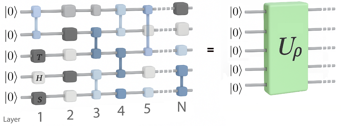
Figure 1: The quantum state emitted by the source is modeled as a concrete sequence of gate instructions. Starting from the all-zeros state, the circuit produces a final quantum state ρ, equivalent to a unitary operator U????.
Measurement circuits
The next step is to evaluate all eight correlation terms appearing in the Svetlichny inequality (Figures 1 and 2). Each term corresponds to a specific choice of local spin measurements. On a quantum computer, we implement these measurements through qubit rotations. In practice, this requires preparing eight separate circuits, one for each correlation term, and sampling their outcomes to compute each E_i.
Given a state ρ generated by a circuit, the mean value of the Svetlichny operator depends on the orientation of local spin angles [7]. We first determine the angles that maximize this value using the SVL() function, then generate the eight measurement circuits with SVL_circuits():
# For each state, compute optimal measurement angles
angles = SVL(circuit)

# Generate the eight circuits and their Svetlichny-inequality coefficients
measurement_circuits, coefficients = SVL_circuits(circuit, angles)

# Store in a dictionary: circuits + coefficients for this state
circuits_for_backends.append({
    'signed_circuits': measurement_circuits,
    'coefficients': coefficients
})
Each entry in circuits_for_backends is a dictionary containing the eight circuits (each combining state preparation with rotations along optimal directions) and the coefficient each correlation term carries in the inequality. Once this list is built, we can submit jobs to either a local simulator or a real QPU.
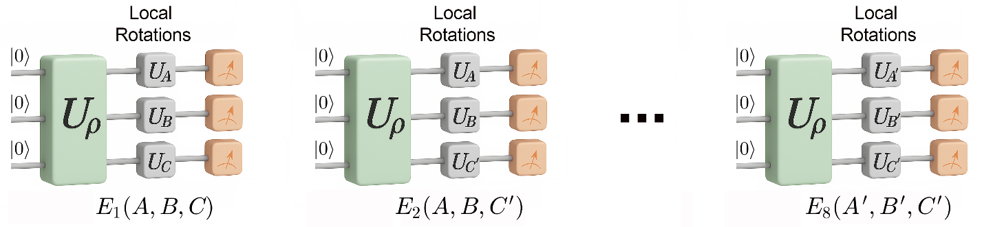
Figure 2: Each correlation term is modeled by the composition of a state-preparation circuit and a measurement layer of local rotations, specified by the computed angles.
Computing the mean value of the Svetlichny operator
Once the correlation circuits are defined, we run them and post-process the results to compute the Svetlichny operator mean value. On a local simulator:
device = LocalSimulator()
num_shots = 1000
If using a noise model, specify the density-matrix simulator:
device = LocalSimulator(backend="braket_dm")The run_test() function in the notebook handles execution and post-processing. For each of the eight circuits, it computes the expectation value using parity-based sampling:
correlations = []

for i in range(len(test["signed_circuits"])):
    p_plus = 0
    p_minus = 0
    input_circuit = test["signed_circuits"][i][0].copy()

    if noise == "True":
        circuit = noise_model.apply(input_circuit)
    else:
        circuit = input_circuit

    task = device.run(circuit, shots=num_shots)
    result = task.result()
    counts = result.measurement_counts

    for key in counts:
        count = key.count("1")
        if (-1)**(count) < 0:
            p_minus += counts[key] / num_shots
        else:
            p_plus += counts[key] / num_shots

    pre_term = p_plus - p_minus
    term = (test["signed_circuits"][i][1]) * pre_term
    correlations.append(term)

svet_value = np.abs(sum(correlations))
print(f"Obtained: {svet_value}, Ideal: {test['Theoretical_violation']}")
The algorithm assigns each measurement outcome a sign based on the parity of “1”s in the bitstring, accumulates p_plus and p_minus, and computes the expectation value for each correlation term. The signed sum gives the Svetlichny operator mean value. A result exceeding 4 confirms GMNL.
Running on a QPU
To run on actual quantum hardware, submit the eight circuits as a batch. After setting up the device and Amazon S3 storage location:
device = AwsDevice("arn:aws:braket:us-east-1::device/qpu/ionq/Forte-1")
num_shots = 1000

my_bucket = "amazon-braket-your-bucket-name"
my_prefix = "IonQ"
s3_location = (my_bucket, my_prefix)

device.run_batch(test_list, s3_location, shots=num_shots)
After retrieving results from Amazon S3, post-processing follows the same procedure: compute expectation values for each correlation term, apply their inequality coefficients, and sum to estimate the mean value of the Svetlichny operator. The run_test() function can be adapted for your own experiments; see the notebook comments for details.
Assessing the performance of quantum processors: an example
Multiple vendors now offer QPUs, both as commercial hardware and as cloud-based services. In the noisy intermediate-scale quantum (NISQ) era, however, performance can vary significantly. Differences appear even when comparing devices with identical architectures, replicas of the same model, the same device at different times, or different qubit subsets within a single processor.
GMNL tests can assess whether a processor functions correctly, helping users decide which devices to use and providing a quantitative benchmark. These tests have distinctive features:
- From foundations to technology: The test is rooted in fundamental physics, providing a principled certification of quantum behavior.
- Whole-register probe: It tests an entire register of qubits simultaneously, rather than isolated qubits or pairs.
- Contextuality: The method establishes correlations across distinct, incompatible measurement contexts, functioning as a test of quantum contextuality that leverages non-Clifford resources.
Figure 3 illustrates results for GHZ states on IonQ Aria-1 and IQM Garnet processors. The plots show the degree of Svetlichny-inequality violation for systems of increasing size, from two to five qubits. Two key points emerge: (i) the expected theoretical violation grows with qubit count, since larger GHZ states display stronger multipartite correlations; (ii) the processors perform differently, revealing how hardware noise and architecture affect the ability to demonstrate GMNL.
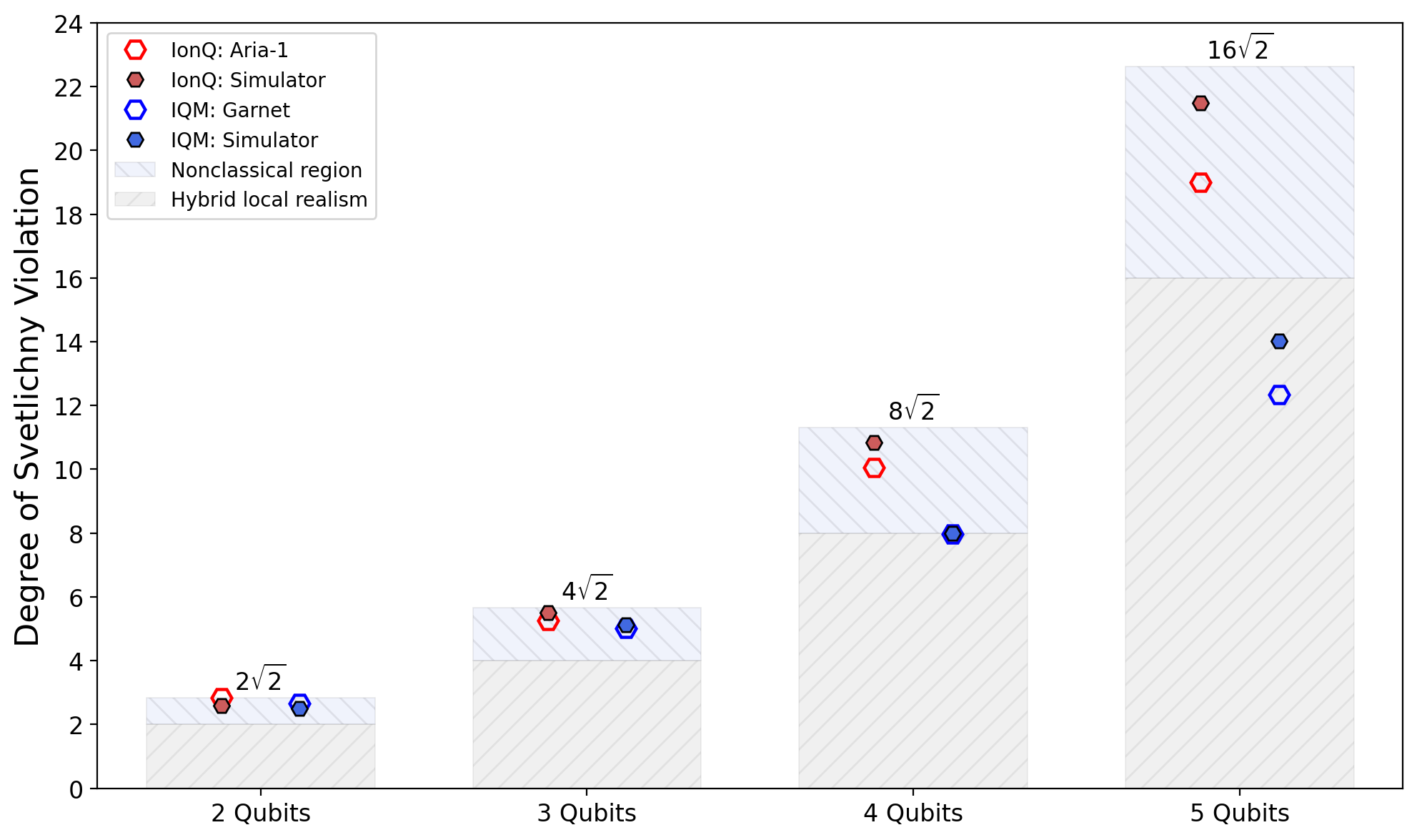
Figure 3: Comparison of Svetlichny inequality violation across IonQ Aria-1 and IQM Garnet processors for 2–5 qubit GHZ states, including local simulator baselines
Conclusion
In this post, we have shown how to demonstrate GMNL on quantum processors using Amazon Braket. After explaining the theory behind genuine multipartite non-locality, we described the implementation steps: state preparation, construction of measurement circuits, and computation of the mean value of the Svetlichny operator. We provided worked-out example code and demonstrated the methodology on IonQ and IQM processors, highlighting its relevance as a benchmarking and calibration tool.
To get started:
- Download the companion notebook and run GMNL tests on the local simulator
- Try different QPUs on Amazon Braket to compare hardware performance
- Extend the analysis to larger systems using the Mermin inequality [8] implementation in the notebook
For more information, visit the Amazon Braket documentation and the Amazon Braket examples repository.
References
[1] Bell, J.S., 1964, “On the Einstein-Podolsky-Rosen paradox”, Physics 1, 195–200; reprinted in Bell 1987b [2004], 14–21.
[2] Einstein, A., Podolsky, B., and Rosen, N., 1935, “Can quantum-mechanical description of physical reality be considered complete?”, Phys. Rev. 47, 777 –780.
[3] Clauser, J.F., Horne, M.A., Shimony and Holt, R.A., 1969, “Proposed experiment to test local hidden-variable theories”, Phys. Rev. Lett. 23, 880–884.
[4] Marissa Giustina, et al., 2015, “Significant-Loophole-Free Test of Bell’s Theorem with Entangled Photons”, Phys. Rev. Lett. 115, 250401.
[5] Svetlichny, G., 1987, “Distinguishing three-body from two-body non-separability by a Bell-type inequality”, Phys. Rev. D 35, 3066.
[6] Seevinck, M and Svetlichny, G., 2002, “Bell-Type Inequalities for Partial Separability in ????-Particle Systems and Quantum Mechanical Violations”, Phys. Rev. Lett. 89, 060401.
[7] Granda Arango, A. C., Holik, F. H., Giuntini, R., Freytes, H. and Sergioli, G., 2025, “Distribution of nonlocality on quantum random circuits”, Phys. Rev. A 112, 062427.
[8] Mermin, N. D., 1990, “Extreme quantum entanglement in a superposition of macroscopically distinct states”, Phys. Rev. Lett. 65, 1838.